Version 2.0 of the popular R package ggplot2 was released three weeks ago. When I was reading the release notes, I largely just skipped over this entry under Deprecated features:

• The order aesthetic is officially deprecated. It never really worked, and
  was poorly documented.

After all, something that “never really worked” didn’t seem that important. But last night, I realized I had indeed been using it, and now needed to find a workaround.

Now, it seems to me like this was not a very widely used feature, and most people were therefore already using a better solution to achieve the same goal. So, to demonstrate what I mean, let’s create some dummy data, and count how many occurrences of each weekday there were in each month last year:

library(dplyr)
library(ggplot2)
library(lubridate)

year_2015 <- data_frame(date=seq(from=as.Date("2015-01-01"), to=as.Date("2015-12-31"), by="day")) %>%
  mutate(month=floor_date(date, unit="month"), weekday=weekdays(date)) %>%
  count(month, weekday)
year_2015

Source: local data frame [84 x 3]
Groups: month [?]

        month   weekday     n
       (date)     (chr) (int)
1  2015-01-01    Friday     5
2  2015-01-01    Monday     4
3  2015-01-01  Saturday     5
4  2015-01-01    Sunday     4
5  2015-01-01  Thursday     5
6  2015-01-01   Tuesday     4
7  2015-01-01 Wednesday     4
8  2015-02-01    Friday     4
9  2015-02-01    Monday     4
10 2015-02-01  Saturday     4
..        ...       ...   ...

year_2015 %>%
  ggplot(aes(x=month, y=n, fill=weekday)) +
  geom_area(position="stack")

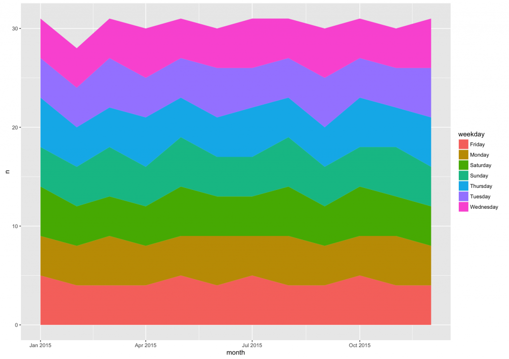
With weekday being character data, by default it is ordered alphabetically, from Friday to Wednesday. But since weekdays of course have a natural order, we can honor that with an ordered factor:

year_2015_factor <- year_2015 %>%
  mutate(weekday=factor(weekday, levels=c("Monday", "Tuesday", "Wednesday",
    "Thursday", "Friday","Saturday", "Sunday"), ordered=TRUE))

year_2015_factor %>%
  ggplot(aes(x=month, y=n, fill=weekday)) +
  geom_area(position="stack")

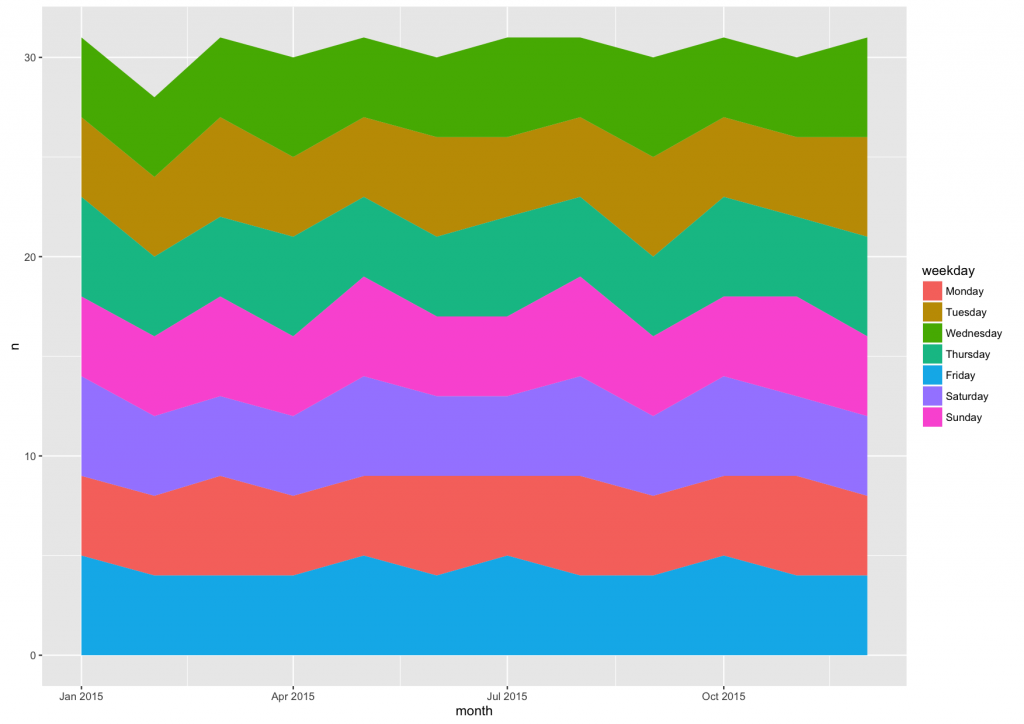
That takes care of the order in the legend, but not in the plot itself. Prior to version 2.0, it was possible to define the plotting order with the order aesthetic:

year_2015_factor %>%
  ggplot(aes(x=month, y=n, fill=weekday, order=-as.integer(weekday))) +
  geom_area(position="stack")

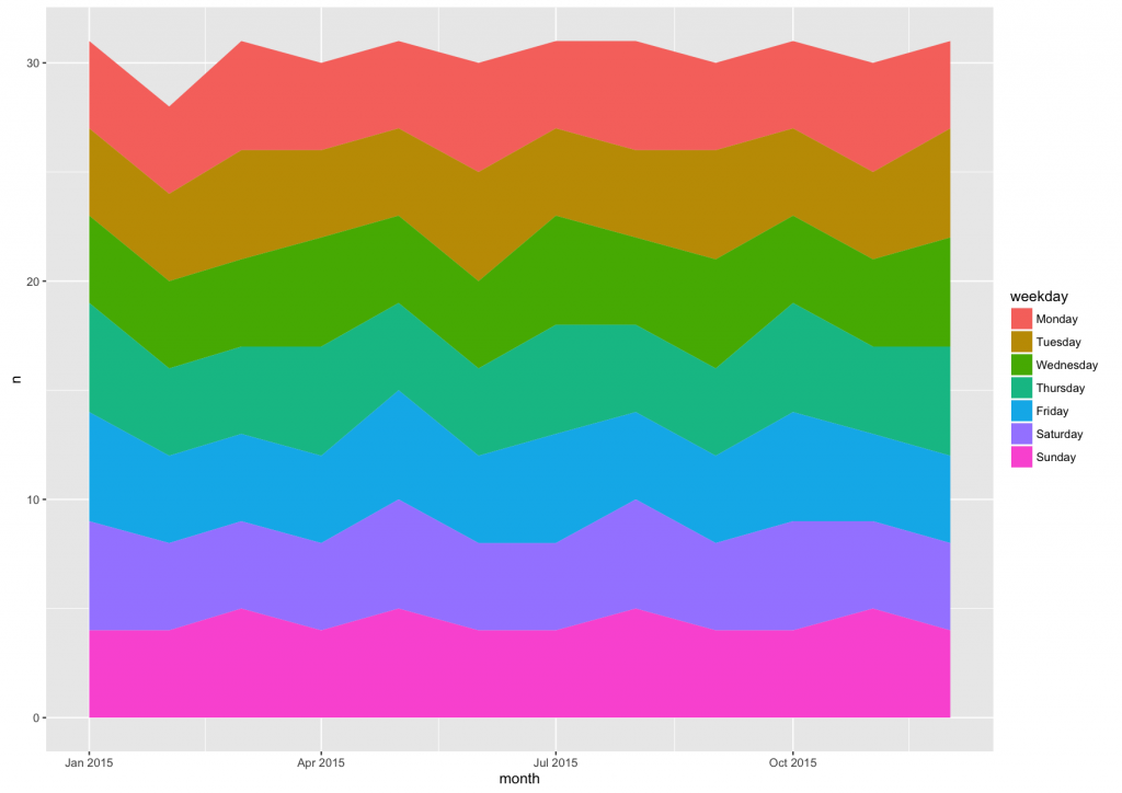
However, that does not work anymore in version 2.0. As I said above, it seems to me that few people were really using the order aesthetic, and most were probably just taking advantage of the fact that the plotting order is the same order in which the data is stored in the data.frame. In this case, it was the alphabetical order as a consequence of using count(). So, let’s re-order the data.frame and plot again:

year_2015_factor %>%
  ungroup() %>%
  arrange(-as.integer(weekday)) %>%
  ggplot(aes(x=month, y=n, fill=weekday)) +
  geom_area(position="stack")

There we go. Now both the plot and the legend are in the same, natural order.

That’s one way to solve the case where I had been using the order aesthetic. I’m not sure if it applies to all other scenarios and geoms as well.