ilari.scheinin.fi

ggplot 2.0 and the missing order aesthetic

by Ilari Scheinin Posted on January 8, 2016

Version 2.0 of the popular R package ggplot2 was released three weeks ago. When I was reading the release notes, I largely just skipped over this entry under Deprecated features:

The order aesthetic is officially deprecated. It never really worked, and
was poorly documented.

After all, something that “never really worked” didn’t seem that important. But last night, I realized I had indeed been using it, and now needed to find a workaround.

Now, it seems to me like this was not a very widely used feature, and most people were therefore already using a better solution to achieve the same goal. So, to demonstrate what I mean, let’s create some dummy data, and count how many occurrences of each weekday there were in each month last year:

library(dplyr)
library(ggplot2)
library(lubridate)

year_2015 <- data_frame(date=seq(from=as.Date("2015-01-01"), to=as.Date("2015-12-31"), by="day")) %>%
  mutate(month=floor_date(date, unit="month"), weekday=weekdays(date)) %>%
  count(month, weekday)
year_2015

Source: local data frame [84 x 3]
Groups: month [?]

        month   weekday     n
       (date)     (chr) (int)
1  2015-01-01    Friday     5
2  2015-01-01    Monday     4
3  2015-01-01  Saturday     5
4  2015-01-01    Sunday     4
5  2015-01-01  Thursday     5
6  2015-01-01   Tuesday     4
7  2015-01-01 Wednesday     4
8  2015-02-01    Friday     4
9  2015-02-01    Monday     4
10 2015-02-01  Saturday     4
..        ...       ...   ...

year_2015 %>%
  ggplot(aes(x=month, y=n, fill=weekday)) +
  geom_area(position="stack")

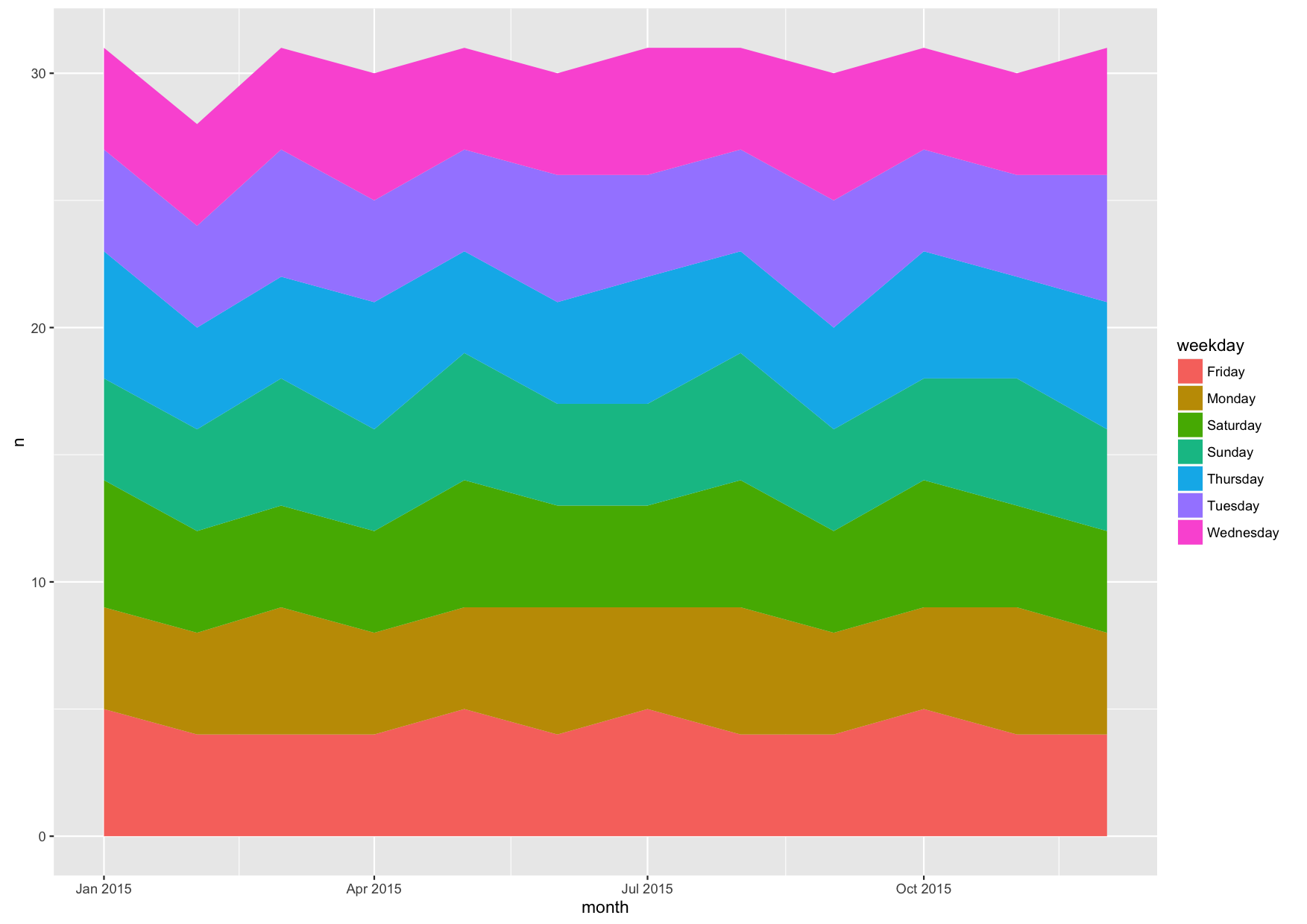
With weekday being character data, by default it is ordered alphabetically, from Friday to Wednesday. But since weekdays of course have a natural order, we can honor that with an ordered factor:

year_2015_factor <- year_2015 %>%
  mutate(weekday=factor(weekday, levels=c("Monday", "Tuesday", "Wednesday",
    "Thursday", "Friday","Saturday", "Sunday"), ordered=TRUE))

year_2015_factor %>%
  ggplot(aes(x=month, y=n, fill=weekday)) +
  geom_area(position="stack")

That takes care of the order in the legend, but not in the plot itself. Prior to version 2.0, it was possible to define the plotting order with the order aesthetic:

year_2015_factor %>%
  ggplot(aes(x=month, y=n, fill=weekday, order=-as.integer(weekday))) +
  geom_area(position="stack")

However, that does not work anymore in version 2.0. As I said above, it seems to me that few people were really using the order aesthetic, and most were probably just taking advantage of the fact that the plotting order is the same order in which the data is stored in the data.frame. In this case, it was the alphabetical order as a consequence of using count(). So, let’s re-order the data.frame and plot again:

year_2015_factor %>%
  ungroup() %>%
  arrange(-as.integer(weekday)) %>%
  ggplot(aes(x=month, y=n, fill=weekday)) +
  geom_area(position="stack")

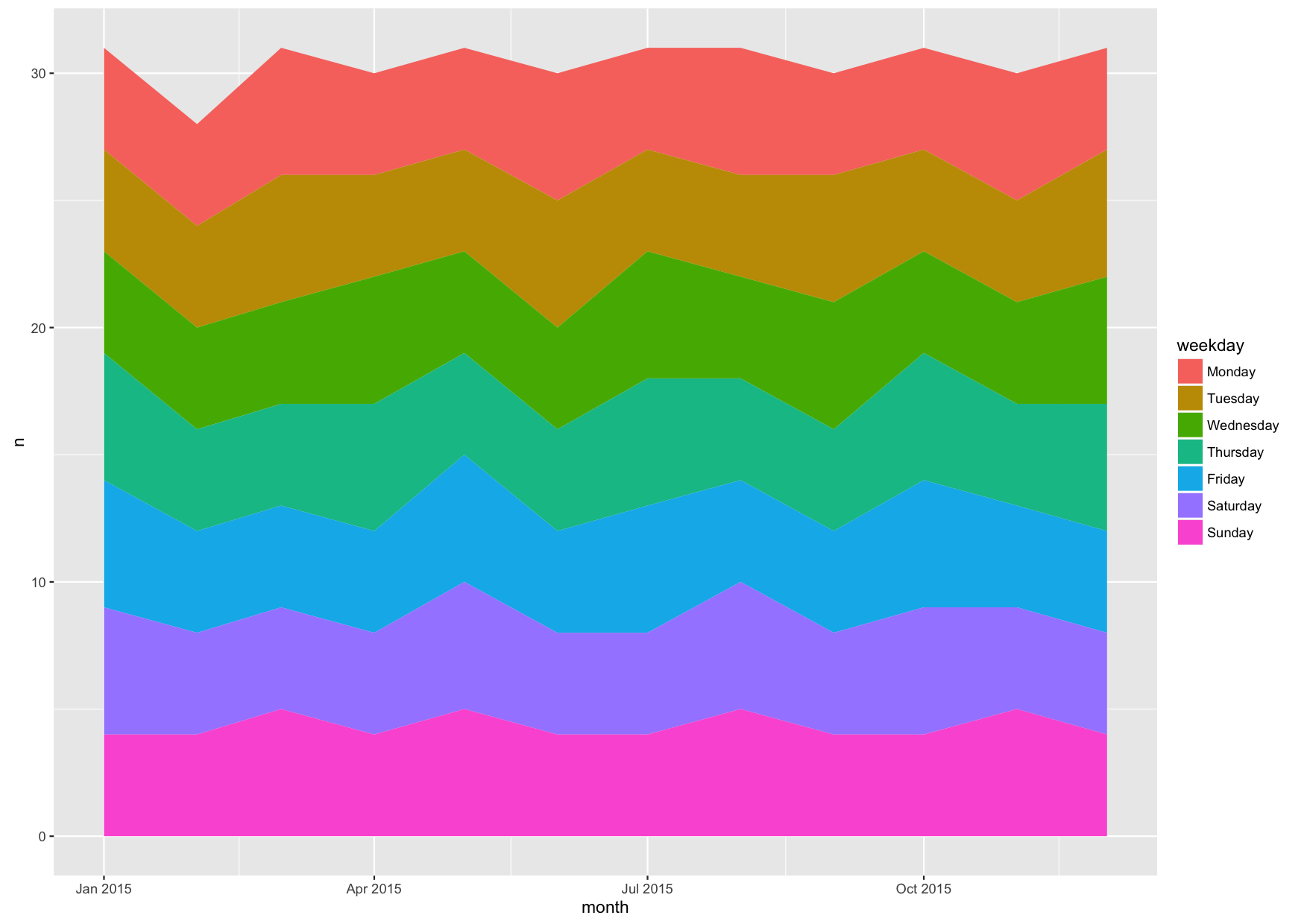
There we go. Now both the plot and the legend are in the same, natural order.

That’s one way to solve the case where I had been using the order aesthetic. I’m not sure if it applies to all other scenarios and geoms as well.

Posted in R | Comments Off

What I Did at the Recurse Center

by Ilari Scheinin Posted on July 8, 2015

Last spring, I spent three months at the Recurse Center, which is like a writers’ retreat for programmers. People from all over the world and with very different backgrounds go there to become better programmers. It’s a great environment for self-learning and collaborating with others. Here I’ll briefly outline what I worked on during that time.

For the past ten years, my number one tool at work as been R. As I’ve been focused on cancer research and chromosomal aberrations, also the packages I’ve used have been from this area (especially Bioconductor). For the three months at RC, I decided to work on broadening my skillset to more general-purpose data science tools.

I still worked mostly in R, and learned to use data manipulation packages like data.table (for more efficiency and modifying data in place) and dplyr (more expressive/logical/readable code, at least for someone like me with background in SQL). For visualizations, I learned how to use ggplot2, how to make interactive apps with shiny, and how to draw maps with ggmap and leaflet. And regarding machine learning, I learned how to use the caret package’s unified interface to train and tune various statistical models. I also took Stanford’s online course on Statistical Learning.

To get to know these packages, I worked on three little projects: how different neighborhoods in New York City vary in their Citi Bike usage patterns, what data from the Moves app tells about how I move and where I’ve been, and also made a prediction on who would win the Stanley Cup.

In addition to working with R, I brushed up my Python skills completing the exercises available at Dataquest. I got to know the very basics of libraries like NumPy, pandas, and matplotlib, as my previous Python experience was only from writing basic utility scripts and not really any type of data analysis.

I also listened to many excellent talks on topics such as public speaking, network protocols, UNIX process model and shell programming, Docker/containerization (and updated the server this website is hosted at to use systemd containers), immutability, hashes, and whether artificial intelligence is a threat or not. Books I read included An Introduction to Statistical Learning, ggplot2 – elegant graphics for data analysis, and The Second Machine Age.

In general, my experience at RC was very positive. I learned a lot and was surrounded with very smart people who I could always ask for advice and guidance. To anyone contemplating a batch I would say go.

Posted in Uncategorized | Comments Off

Predicting the Stanley Cup Champion

by Ilari Scheinin Posted on July 8, 2015

When I was at the Recurse Center, I wanted to try the caret package for R. It provides a unified interface for training various types of classification and regression models, and parameter tuning through resampling. I needed a project to work on, and since I love hockey and the Stanley Cup playoffs were just starting, it was a natural choice.

The source code is all on GitHub, and is split into four R Markdown documents: scrape raw data, process data, train models, and make predictions. I’ll present a short summary here, and more details can be found behind those links. The repository also contains a Makefile to replicate the analysis. Random seeds are specified in the code to make it fully reproducible.

First, I used the nhlscrapr package to scrape play-by-play data from NHL.com starting from the 2002-2003 season. Then, I used dplyr to calculate some summary statistics. For each game, I calculated the following statistics for both the home and away teams:

the proportion of goals scored, i.e. “goals scored / (goals scored + goals against)”
the proportion of shots
the proportion of faceoffs won
the proportion of penalties
power play, i.e. “power play goals scored / penalties for the other team”
penalty kill, i.e. “power play goals against / penalties for own team”

I’m sure many more useful predictor variables could be derived from the play-by-play data, which in turn would result in more accurate predictions. But since this was mainly an exercise to try out caret, these variables will suffice for now.

For each season, I then calculated the average performance of each team, separately for when they were playing at home and on the road. Here’s an example of away performance for six teams from the 2002-2003 season:

season	team	goals	shots	faceoffs	penalties	pp	pk
20022003	ANA	0.480	0.477	0.544	0.517	0.159	0.095
20022003	ATL	0.433	0.434	0.467	0.504	0.147	0.139
20022003	BOS	0.422	0.503	0.481	0.555	0.137	0.103
20022003	BUF	0.416	0.482	0.493	0.526	0.118	0.119
20022003	CAR	0.384	0.492	0.512	0.514	0.105	0.169
20022003	CBJ	0.376	0.432	0.472	0.511	0.110	0.104

Next, I took the outcomes of all playoff series from the past 11 seasons, and calculated two deltas to be used as explanatory variables. I calculated the difference between the home team’s home performance and the away team’s away performance, and also the home team’s away performance and the away team’s home performance. This was to capture how the two teams would perform at the two arenas for the series.

I then used caret to train five different types of statistical models on this training data. The methods I included were generalized linear model, linear discriminant analysis, neural network, random forest, and support vector machine with a linear kernel. For each, model parameters were tuned with 10-fold cross-validation, which was repeated 10 times. Parameter values with the best overall accuracy were used to fit the final model with all of the training data.

For my predictions, instead of picking just one of the five fitted models, I used all of them. For each playoff series, I used a majority vote from all five models to pick the winner. (That’s why I fitted an odd number of models.) The predictions are below, with the predicted winner in bold:

Round 1

Pittsburg Penguins at New York Rangers
Ottawa Senators at Montreal Canadians
Detroit Red Wings at Tampa Bay Lightning
New York Islanders at Washington Capitals
Winnipeg Jets at Anaheim Ducks
Minnesota Wild at St. Louis Blues
Chicago Blackhawks at Nashville Predators
Calgary Flames at Vancouver Canucks

Round 2

New York Islanders at New York Rangers
Tampa Bay Lightning at Montreal Canadians
Calgary Flames at Anaheim Ducks
Chicago Blackhawks at St. Louis Blues

Round 3 – Conference Finals

Montreal Canadians at New York Rangers
Chicago Blackhawks at Anaheim Ducks

Round 4 – Stanley Cup Finals

Chicago Blackhawks at New York Rangers

My prediction for the 2015 Stanley Cup Champion was Chicago Blackhawks.

To be clear, this blog entry was posted after the playoffs were already over. The explanatory text in the R Markdown documents was also written during the playoffs. But the same prediction as presented above can be seen in this GitHub commit (and the same HTML document on RawGit) from April 23rd. This was not before the playoffs started (April 15th), but when the first round was 3-4 games in, depending on the series.

Validation Set

And since the playoffs are in fact already over, it means that the natural validation set is also available. Chicago Blackhawks did end up winning the Cup, but how did I do otherwise? Below are the predictions again, now together with the real outcomes. And since an incorrect prediction in one round leads to wrong pairs on the subsequent rounds, I have added in the series that actually ended up happening. (I made a prediction for all possible games that could happen, but only presented the resulting bracket here.) These added ones are in italics.

Round 1

Pittsburg Penguins at New York Rangers – correct
Ottawa Senators at Montreal Canadians – correct
Detroit Red Wings at Tampa Bay Lightning – correct
New York Islanders at Washington Capitals – INCORRECT
Winnipeg Jets at Anaheim Ducks – correct
Minnesota Wild at St. Louis Blues – INCORRECT
Chicago Blackhawks at Nashville Predators – correct
Calgary Flames at Vancouver Canucks – correct

Round 2

Washington Capitals at New York Rangers – correct
Tampa Bay Lightning at Montreal Canadians – INCORRECT
Calgary Flames at Anaheim Ducks – correct
Minnesota Wild at Chicago Blackhawks – correct

Round 3 – Conference Finals

Tampa Bay Lightning at New York Rangers – INCORRECT
Chicago Blackhawks at Anaheim Ducks – correct

Round 4 – Stanley Cup Finals

Chicago Blackhawks at Tampa Bay Lightning – correct

Overall, my accuracy was 11 out of 15, which is 73%.

An obvious follow-up from here could be to look at each of the five different models (generalized linear model, linear discriminant analysis, neural network, random forest, and support vector machine with a linear kernel) and compare their accuracies against each other.

Posted in R, sports | Comments Off

Where I’ve Been and How?

by Ilari Scheinin Posted on July 8, 2015

I have been running the Moves app on my phone for almost two years. I guess its main idea is to be an activity tracker; it’ll tell you how much you’ve walked, ran, or ridden a bike, without you having to remember to turn it on before starting an “activity”. But for me the main point isn’t as much the activity part as it is the tracking part. Without me having to do anything, the app silently collects data about my movements in the background. I can then download the accumulated data and play around with it in R.

When I was at the Recurse Center, I needed a little project to work on learning ggplot2 and shiny, and chose to do a remake of this old blog post on the shares of different modes of transportation I use. The end result is packaged into a shiny app, and shows for example that in New York I walked a lot more than I used to while living in Amsterdam or Helsinki, and that last summer I spent a lot of time on boats. A more subtle difference is that in Amsterdam I seemed to use trams only for commuting to work.

I also wanted to try out some mapping with leaflet, and made another app that shows all my movement while I was in New York. If all checkboxes are turned on, four months of data seems to be a bit much to handle performance-wise, and the app becomes slow and sometimes crashes (turns gray and stops responding). Anyways, it was a fun experiment to do.

The source code is available on GitHub.

Posted in cycling, R, transportation | Comments Off

Citi Bikes and Neighborhoods

by Ilari Scheinin Posted on July 8, 2015

New York City has an excellent bike sharing system called Citi Bikes. When I was at the Recurse Center, I frequently used the bikes for commuting. What was annoying though, was that every now and then all the nearby docks were empty by the time I was leaving. I guess this was because it was mostly a residential area, so in the mornings people would grab the bikes and ride them to work, and in the evenings the bikes would flow back. A business district would naturally see the opposite pattern. (I know the operators rebalance bikes between stations, but I don’t know if this happens intra-day or just to correct slower drift patterns.)

In addition to being a convenient way to move around, another nice thing about the system is that they release their ride data publicly. I decided do a little experiment in R. I downloaded all their data and used dplyr to count the number of bikes arriving to and leaving from each station. I did that for each hour of the day and separately for weekdays and weekends.

In order to visualize the patterns, I plotted them with ggmap and made a little shiny app.

To identify neighborhoods with similar usage patterns, I used K-means clustering and put the results in another shiny app. It also contains a plot of the variance explained for assessing a suitable value for K.

The source code is available on GitHub.

Posted in cycling, R, transportation, urban | Comments Off

How I Move

by Ilari Scheinin Posted on October 2, 2014

With 12 full months of Moves data, I thought it would be a fun experiment to make some plots. These show how I move around in terms of time spent and distance traveled, both for relative share of each mode of transport, and for the total time or distance. Flying is excluded.

Posted in cycling, R, transportation, Uncategorized | Comments Off

A single dream is more powerful than a thousand realities

by Ilari Scheinin Posted on March 26, 2014

A single dream is more powerful than a thousand realities
– J.R.R. Tolkien

Is it really? Personally, I prefer reading about things that actually could have happened. And the only thing better than that is things that actually did happen. How Lawrence Oates on Scott’s expedition to the South Pole was slowing the whole group down because of his poor condition, and one morning decided to walk out of the tent into the blizzard to help others survice. “I’m just going outside and may be some time.”

Or how the former NHLer Theo Fleury describes the tops and bottoms of his life. How being sexually abused by his coach as a teenager made him a living wreck, who simply could not go home and to bed while it was still dark, because that’s where the bad things had happened. Instead, the only way to get through the nights was to stay out drinking, sniffing coke, and going to casinos and stripclubs. “You know that picture The Scream, by Edvard Munch? It is a picture of me.” Or after all this, how it felt like to be on the ice after Team Canada had just won Olympic Gold in Salt Lake City, and he saw his own parents in the stands going berserk. “Here was a guy who had barely acknowledged my existence when I was growing up, and now he looked like like he was in Rome, cheering for the gladiators. And I realized that I was that gladiator. I was the hero he was screaming for. He looked right at me, and I saw admiration. It blew me away. It was the greatest feeling ever.”

Or how one of the most violent storms in history hit the 1979 Fastnet Race, and after their boat had — once again — been knocked over by the big waves, Nick Ward regained conciousness in the water and climbed back on board with the help of his harness only to find one of his crewmates dead and the others disappeared with the lifeboat. How he spent the next day fighting the storm, climbing back on board after more knockdowns, trying to keep his sanity by talking to his dead mate, and bailing water out of the sinking boat until he could no longer move and no longer keep himself conscious. Until he was saved. “‘Gerry, look, mate, look… it’s a helicopter, it’s a Sea King.’ And in my bemused state I pointed to the sky and wept.”

Maybe I lack imagination, but to me, these realities feel more powerful than a thousand dreams.

Posted in literature | Comments Off