Update April 12, 2018: This post is from spring 2017, so the results reflect statistics up to season 2016–2017. I have now re-run the analysis including data from season 2017–2018, and updated results are available here. Methodology is unchanged, so everything below is still an accurate description of how the analysis was performed.
In this post I will look at the question of who have been the best shooters in the NHL. The metric I will use is the shooting percentage, which is the number of goals scored divided by the number of shots on goal. To deal with two issues that will be explained in the next section, I will use a technique called Bayesian multilevel modeling. If that sounds complicated, fear not; it works kind of the same way as human intuition.
After Jake Guentzel scored his first NHL career goal during his first shift in his first game with his first shot, his shooting percentage was 100%. But no reasonable human being would say based on that alone that he was the best shooter of all times with that flawless record. Instead, to evaluate a new player, one tends to start with a vague assumption that their shooting ability is probably somewhat average, but can also be higher or lower. Then, as more and more evidence builds up, that assumption is updated, which leads to a more and more precise picture. This is essentially what “Bayesian modeling” means; start with a prior expectation and update it with the data you have.
There are many ways we can come up with that prior expectation. It could be the average shooting percentage of all players in the league, or defined more narrowly. Depending on the situation, we could for example look only at players who shoot from the right. Or players who are first-round draft picks. Or use the information we have on player position, and assess forwards and defencemen separately. After all, on average forwards do score more goals and in general shoot from much closer to the opponent’s net than defencemen. Here, the use of such a hierarchy, players grouped according to their position, is the “multilevel modeling” part.
When these two are put together, what Bayesian multilevel modeling means for this post is that I will use historical player statistics to estimate average performance separately for forwards and defencemen, and use this average as the starting point to evaluate each individual player. The more evidence there is for any given player, the further away we are ready to move from the average.
This post contains all the code needed to perform the analysis with R and Stan, but the code sections can be freely skipped over if one is not interested in them. Impatient readers can also skip directly to the results section, or just look at the full result table.
Data
Our data consists of the number of goals scored and shots on goal for each player for each regular season. NHL started to count shots on goal for season 1967–1968, so our data spans from that season to the just finished one 2016–2017. Here’s an excerpt of the first ten data rows. 1
| player | position | season | shots | goals | |
|---|---|---|---|---|---|
| 1 | Antti Aalto | forward | 1997-1998 | 1 | 0 |
| 2 | Antti Aalto | forward | 1998-1999 | 61 | 3 |
| 3 | Antti Aalto | forward | 1999-2000 | 102 | 7 |
| 4 | Antti Aalto | forward | 2000-2001 | 18 | 1 |
| 5 | Spencer Abbott | forward | 2013-2014 | 2 | 0 |
| 6 | Spencer Abbott | forward | 2016-2017 | 1 | 0 |
| 7 | Justin Abdelkader | forward | 2007-2008 | 6 | 0 |
| 8 | Justin Abdelkader | forward | 2008-2009 | 2 | 0 |
| 9 | Justin Abdelkader | forward | 2009-2010 | 79 | 3 |
| 10 | Justin Abdelkader | forward | 2010-2011 | 129 | 7 |
We can aggregate this by player to get raw career shooting percentages.
| player | position | career | shots | goals | raw | |
|---|---|---|---|---|---|---|
| 1 | Antti Aalto | forward | 1997–2001 | 182 | 11 | 6.04% |
| 2 | Spencer Abbott | forward | 2013– | 3 | 0 | 0.00% |
| 3 | Justin Abdelkader | forward | 2007– | 964 | 85 | 8.82% |
| 4 | Pontus Aberg | forward | 2016– | 12 | 1 | 8.33% |
| 5 | Dennis Abgrall | forward | 1975–1976 | 9 | 0 | 0.00% |
| 6 | Ramzi Abid | forward | 2002–2007 | 112 | 14 | 12.50% |
| 7 | Thommy Abrahamsson | defenceman | 1980–1981 | 66 | 6 | 9.09% |
| 8 | Noel Acciari | forward | 2015– | 33 | 0 | 0.00% |
| 9 | Doug Acomb | forward | 1969–1970 | 0 | 0 | |
| 10 | Keith Acton | forward | 1979–1994 | 1,690 | 226 | 13.37% |
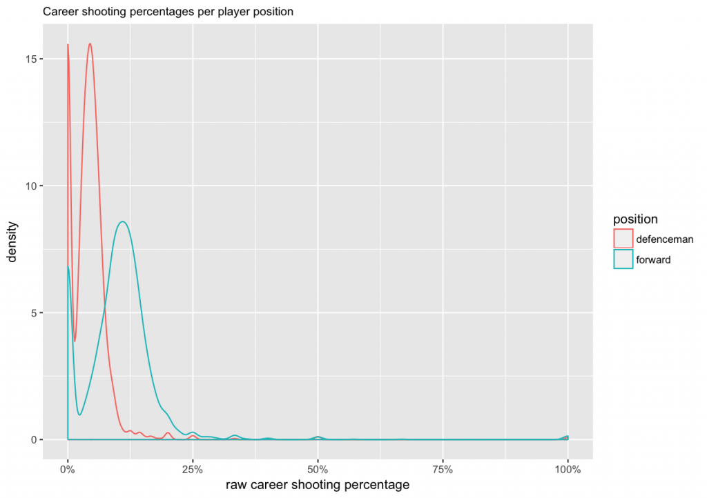
To get an idea of common values for raw career shooting percentage, we make a density plot and separate between forwards and defencemen.
From the plot we can see that:
1. Defencemen tend to have lower shooting percentages than forwards (averages of about 4.5% and 11%).
2. There are big peaks at zero, which represent players who have never scored a goal (and who might also have a very small number of shots on goal).
3. There are also small peaks at 100%, 50%, 33%, etc, which represent players who have a small number of shots on goal, but who got lucky and scored.
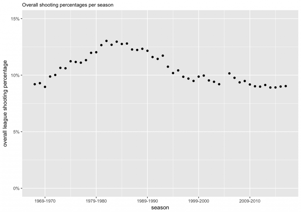
Points 2. and 3. above are the first reason why we use the modeling approach. It will give us with a way to assess players for whom we have little data. The second reason is the fact that the gameplay in the NHL has changed over the years. Nowadays the game is faster, and players have less time and less space to maneuver with the puck and to score. Also, a lot more attention is paid to goaltending, and goalies receive more training and coaching on their technique than in the old days. To assess this change over time, we can plot the overall league shooting percentages per season.
From the plot we can see that the average shooting percentage has indeed changed over time, and was the highest in the 1980s.
Model
For every shot on goal, there are two possible outcomes: a goal or no goal. When we count the number of goals scored (successes) from some number of shots on goal (trials), in statistics this is represented with the binomial distribution. In addition to the number of trials, the number of successes depend on the probability of success for each trial, which here represents the player’s shooting ability, or skill. This probability is assumed to be the same for each trial, which is naturally not really true here. In reality, the probability varies from play to play, and is affected by factors such as distance, proximity of other players, positioning of the goalie, and so forth. But here we make an oversimplification and assume that each player has a constant probability of success that depends on their skill. For any given player on any given season, the number of goals scored is therefore distributed as:
goals scored ~ binomial(shots on goal, skill of player)
Another oversimplification we are going to make is that we assume players’ skills to stay constant not only within a season, but all through their careers. Again, in real life young players develop and get better, and before older players retire, their performance generally shows some decline. But here we are interested in ranking the best shooters, and want to be able to compare players across time, for example current players to those who played in the 1980s. Therefore, we will define the probability of success as the player’s skill minus the difficulty of the season.
goals scored ~ binomial(shots on goal, skill of player – difficulty of season)
The seasonal difficulty represents the combined effect of all other factors besides the player’s skill, such as goaltending, overall gameplay, and so on. We are able to combine these effects, because most players’ careers have spanned multiple seasons. This allows us to fit a model that finds an innate skill for each player (that stays constant throughout their career) and separately captures an estimate for seasonal difficulty.
We fit this model with Stan.
Evaluation
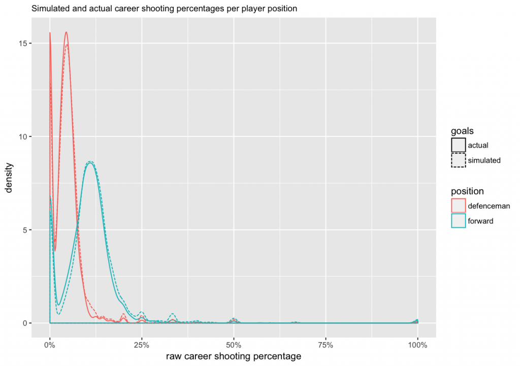
Now that we have fitted our model, we would like to evaluate if it makes sense. One way to approach this is with a simulation. We can use the model (players’ skills, and seasons’ difficulties) and the historical number of shots on goal to generated a simulated set of goals scored. Then we can visualize the actual and simulated numbers, and see if they behave similarly. Let’s start with the same density plot we used above to evaluate typical raw career shooting percentages for forwards and defencemen. Actual results are shown with a solid line, and the simulation results with a dashed line. Ideally, they should be close to each other.
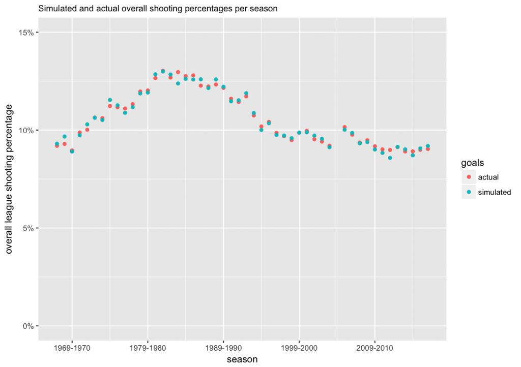
We will also re-create the plot we used above for overall league shooting percentages per season. Again, ideally the actual and simulated data points should be close to each other.
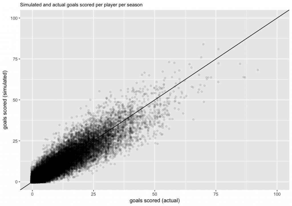
And finally, we will make a scatter plot of actual and simulated goals scored per player per season. Ideally, the cloud of points should be symmetric around the diagonal line.
In the density plot, the fit looks good for defensemen, but for forwards the model seems to slightly overestimate the number of forwards with an average raw shooting percentage (around 11%), and underestimate the number of forwards with low raw shooting percentages. Otherwise the fits seem to be reasonable close. So, let’s look at the results.
Results
When we fit the model, two things happen to the original raw career shooting percentages. First, they are shrunk towards the averages defined separately for forwards or defencemen. Second, they are adjusted for the seasonal difficulty. For players with careers during the “easier” seasons, such as in the 1980s, this will reduce their estimated skill. And for players who played during seasons with a higher estimated difficulty, their skill values will see an increase.
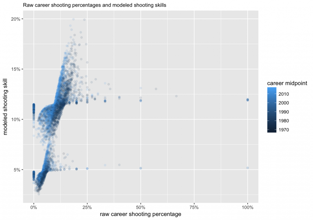
The resulting values, players’ skills, are visualized here together with their raw career shooting percentages.
We can see that among the raw shooting percentages on the x-axis, there are extreme values, such as 0%, 100%, 50%, etc. But on the modeled skill on the y-axis, they have been shrunk to all be between about 2% and 20%. Also visible are the two separate clusters for forwards (around 11%–12%), and defencemen (4%–5%). The shades of blue show how the same raw career shooting percentage results in a higher estimated skill for more recent players compared to the 1970s and 80s.
Finally, below are tables of the top 10 forwards and defencemen, ranked according to their modeled shooting skills.
| player | position | career | shots | goals | raw | model | |
|---|---|---|---|---|---|---|---|
| 1 | Alex Tanguay | forward | 1999–2016 | 1,525 | 283 | 18.56% | 19.96% |
| 2 | Craig Simpson | forward | 1985–1995 | 1,044 | 247 | 23.66% | 19.91% |
| 3 | Steven Stamkos | forward | 2008– | 1,876 | 321 | 17.11% | 19.32% |
| 4 | Andrew Brunette | forward | 1995–2012 | 1,516 | 268 | 17.68% | 18.92% |
| 5 | Sergei Makarov | forward | 1989–1997 | 610 | 134 | 21.97% | 18.66% |
| 6 | John Bucyk | forward | 1967–1978 | 1,723 | 329 | 19.09% | 18.39% |
| 7 | Mark Parrish | forward | 1998–2011 | 1,247 | 216 | 17.32% | 18.17% |
| 8 | Charlie Simmer | forward | 1974–1988 | 1,531 | 342 | 22.34% | 18.14% |
| 9 | Gary Roberts | forward | 1986–2009 | 2,374 | 438 | 18.45% | 17.92% |
| 10 | Ray Ferraro | forward | 1984–2002 | 2,164 | 408 | 18.85% | 17.68% |
| player | position | career | shots | goals | raw | model | |
|---|---|---|---|---|---|---|---|
| 1 | Sandis Ozolinsh | defenceman | 1992–2008 | 1,771 | 167 | 9.43% | 9.55% |
| 2 | Shea Weber | defenceman | 2005– | 2,235 | 183 | 8.19% | 9.24% |
| 3 | Mike Green | defenceman | 2005– | 1,618 | 134 | 8.28% | 9.15% |
| 4 | Lubomir Visnovsky | defenceman | 2000–2015 | 1,532 | 128 | 8.36% | 9.00% |
| 5 | Bobby Orr | defenceman | 1967–1979 | 2,795 | 257 | 9.19% | 8.91% |
| 6 | Marc-Andre Bergeron | defenceman | 2002–2013 | 951 | 82 | 8.62% | 8.88% |
| 7 | Oliver Ekman-Larsson | defenceman | 2010– | 1,134 | 88 | 7.76% | 8.53% |
| 8 | Nick Holden | defenceman | 2010– | 350 | 32 | 9.14% | 8.45% |
| 9 | Tyler Myers | defenceman | 2009– | 737 | 59 | 8.01% | 8.45% |
| 10 | Mark Giordano | defenceman | 2005– | 1,295 | 99 | 7.64% | 8.44% |
Craig Simpson holds the official record for best career shooting percentage, which only counts players with at least 800 shots on goal, with 23.66%. But here he has lost the number one spot to Alex Tanguay, who originally ranked 22nd. Their modeled shooting skills are 19.91% vs. 19.96%. This is is due to the fact that Simpson’s career was in 1985–1995, which according to the model was a less difficult era for goal scoring than Tanguay’s 1999–2016.
There are many such differences between the official career shooting percentage ranking and our modeled one. They can be explored from the full table with 5,574 players. It is by no means the right ranking; it is simply a plausible one given the model and assumptions described above. But compared to the official ranking for career shooting percentage, it does have two benefits. First, it does not omit players with less than 800 career shots on goal. And second, it provides one way to gauge changes in gameplay, and thus facilitate comparisons between players whose careers do not overlap. So, while the model’s assumptions are not exactly realistic (an innate shooting skill that stays constant for the duration of a player’s career), the results can be a useful complement to the official career shooting percentage statistics in some situations.
Centers and left/right wingers are all counted simply as “forwards”. This is because multiple players have played both as centers and wingers. The small number who have played both as forwards and defencemen were excluded from the analysis.↩
